MC3 <- jsonlite::fromJSON("data/MC3.json")Visual analytics process to find similar businesses
Take Home Exercise 3
The objective of this challenge is to utilize the visual analytics process to identify and categorize the products and services offered by companies based on their similarity. To achieve this, we will utilize Topic modeling (LDA), to extract the main objectives from each group. Through this method, we can assign topics to business group based on their product_service description. Subsequently, we will have a closer look on their revenue distribution across different business groups.
Data Import
Load packages
pacman::p_load(jsonlite, tidygraph, ggraph,
               visNetwork, graphlayouts, ggforce,
               skimr, tidytext, tidyverse, SnowballC, hunspell, textstem, udpipe, dplyr, tm, text2vec, topicmodels, widyr, textmineR, topicdoc, fpc, cluster, ggplot2, scales, plotly, wordcloud, RColorBrewer, gridExtra, grid, forcats)
Extracting edges
mc3_edges <- as_tibble(MC3$links) %>%
  distinct() %>%
  mutate(source = as.character(source),
         target = as.character(target),
         type = as.character(type)) %>%
  group_by(source, target, type) %>%
    summarise(weights = n()) %>%
  filter(source!=target) %>%
  ungroup()
Extracting nodes
mc3_nodes <- as_tibble(MC3$nodes) %>%
  mutate(country = as.character(country),
         id = as.character(id),
         product_services = as.character(product_services),
         revenue_omu = as.numeric(as.character(revenue_omu)),
         type = as.character(type)) %>%
  select(id, country, type, revenue_omu, product_services)
Find out similar business groups
Data preparation
Step 1. Address missing values replace character(0) with NA, and drop those NAs
Show code
mc3_nodes <- mc3_nodes %>%
  mutate(product_services = ifelse(product_services == "character(0)", NA, product_services)) %>%
  mutate(product_services = ifelse(product_services == "Unknown", NA, product_services))%>%
  drop_na(product_services)
Step 2: Tokenization and remove non-alphabets
Show code
token_nodes <- mc3_nodes %>%
  unnest_tokens(word,
                product_services)%>%

  mutate(word = str_replace_all(word, "[^a-z]", "")) %>%
  filter(word != "")
Step 3: lemmatization
Show code
token_nodes$word <- lemmatize_words(token_nodes$word)Step 4: remove stopwords
Show code
data("stop_words")
token_nodes <- token_nodes %>%
  anti_join(stop_words)
Step 5: remove words that are not in the dictionary
Show code
token_nodes <- token_nodes %>%
  filter(hunspell_check(word))
Step 6: keep only nouns
Show code
ud_model <- udpipe_download_model(language = "english")
ud_model <- udpipe_load_model(ud_model$file_model)

token_nodes_filter <- udpipe_annotate(ud_model, x = token_nodes$word)
token_nodes_filter <- as.data.frame(token_nodes_filter)
token_nodes_filter <- token_nodes_filter[token_nodes_filter$upos == "NOUN", ]
token_nodes_filter <- token_nodes_filter %>%
  select(lemma, upos) %>%
  distinct(lemma, upos)

token_nodes_table <- left_join(token_nodes, token_nodes_filter, by = c("word" = "lemma")) %>%
  drop_na(upos) %>%
  select(id, country, type, revenue_omu, word)
Step 7: adding custom into stopwords
custom_stop_words <- bind_rows(stop_words, tibble(word = c( "product", "service", "system", "process", "offer", "range", "supply", "solution", "source",
"freelance", "researcher", "management", "component", "manufacturing", "distribution", "tool", "care",
"industry", "service", "raw", "specialty", "home", "item", "specialty", "activity", "control", "line", "production", "prepared", "development", "product", "include", "business", "commercial", "die", "application", "industry", "international", "preparation", "special", "based", "natural",  "building", "build", "personal", "type",  "appliance",  "variety", "head", "ingredient", "series", "smoke", "material"), lexicon = c("en")))

token_nodes_table <- token_nodes_table %>%
  anti_join(custom_stop_words)
Step 8: Retain the words that have a frequency of more than 5.
Show code
word_counts <- token_nodes_table %>%
  count(word, sort = TRUE)

# Filter out words with count less than 5
filtered_table <- word_counts %>%
  filter(n >= 5)

token_nodes_table <- semi_join(token_nodes_table, filtered_table, by = "word")
Visualise the unique words in product service field
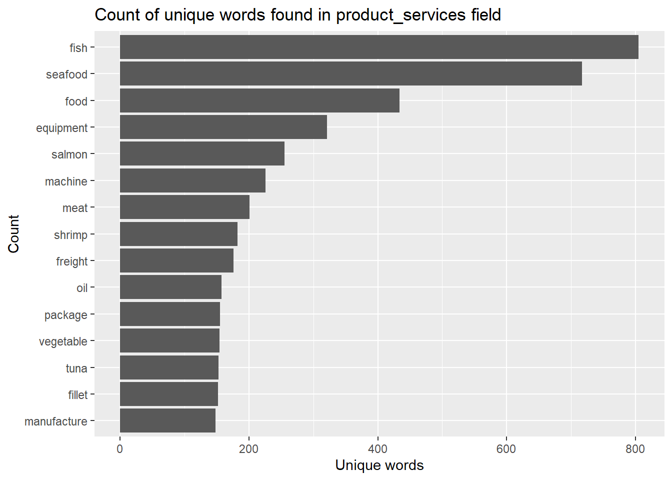
token_nodes_table %>%
  count(word, sort = TRUE) %>%
  top_n(15) %>%
  mutate(word = reorder(word, n)) %>%
  ggplot(aes(x = word, y = n)) +
  geom_col() +
  xlab(NULL) +
  coord_flip() +
      labs(x = "Count",
      y = "Unique words",
      title = "Count of unique words found in product_services field")
LDA
Create a Document-Term Matrix (DTM):
# group the product services keywords of the same company into a row
token_nodes_table <- token_nodes_table %>%
  group_by(id) %>%
  summarise(product_services = paste(word, collapse = " "))

corpus <- Corpus(VectorSource(token_nodes_table$product_services))
nodes_dtm <- DocumentTermMatrix(corpus, control = list(tolower = TRUE, removePunctuation = TRUE, stopwords = TRUE))
dtm_matrix <- as.matrix(nodes_dtm)
Compute Coherence Score
Determining the optimal number of topics based on the highest coherence score suggests that having 6 topics is ideal.
k <- 15
set.seed(1234)
lda_model <- LDA(nodes_dtm, k, method="Gibbs", control=list(iter = 500, verbose = 25))
K = 15; V = 1019; M = 3642
Sampling 500 iterations!
Iteration 25 ...
Iteration 50 ...
Iteration 75 ...
Iteration 100 ...
Iteration 125 ...
Iteration 150 ...
Iteration 175 ...
Iteration 200 ...
Iteration 225 ...
Iteration 250 ...
Iteration 275 ...
Iteration 300 ...
Iteration 325 ...
Iteration 350 ...
Iteration 375 ...
Iteration 400 ...
Iteration 425 ...
Iteration 450 ...
Iteration 475 ...
Iteration 500 ...
Gibbs sampling completed!coherence <- topic_coherence(lda_model, nodes_dtm, top_n_tokens = 10, smoothing_beta = 1)
k_values <- 1:15
coherence_table <- data.frame(k = k_values, "coherence score" = coherence)
coherence_table k coherence.score
1 1 -100.22628
2 2 -217.74938
3 3 -84.48798
4 4 -191.00726
5 5 -198.63736
6 6 -84.15613
7 7 -226.50561
8 8 -202.58051
9 9 -131.86465
10 10 -198.55230
11 11 -192.52602
12 12 -125.37263
13 13 -195.44364
14 14 -169.19899
15 15 -175.96578Build LDA for topic modelling
K <- 6
set.seed(1234)
# compute the LDA model, inference via 1000 iterations of Gibbs sampling
topicModel <- LDA(nodes_dtm, K, method="Gibbs", control=list(iter = 500, verbose = 25))
K = 6; V = 1019; M = 3642
Sampling 500 iterations!
Iteration 25 ...
Iteration 50 ...
Iteration 75 ...
Iteration 100 ...
Iteration 125 ...
Iteration 150 ...
Iteration 175 ...
Iteration 200 ...
Iteration 225 ...
Iteration 250 ...
Iteration 275 ...
Iteration 300 ...
Iteration 325 ...
Iteration 350 ...
Iteration 375 ...
Iteration 400 ...
Iteration 425 ...
Iteration 450 ...
Iteration 475 ...
Iteration 500 ...
Gibbs sampling completed!Word Cloud
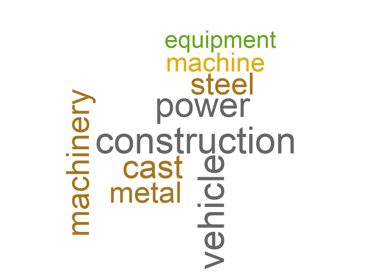
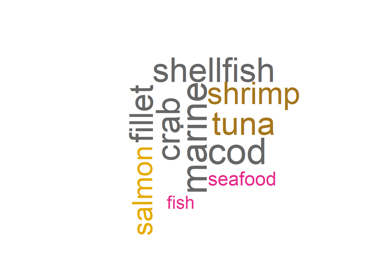
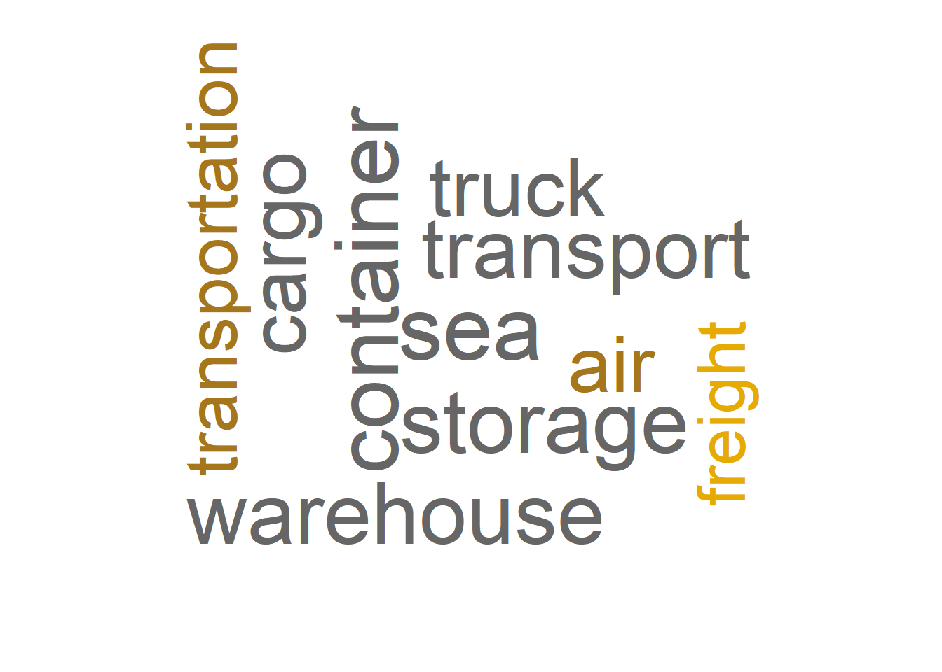
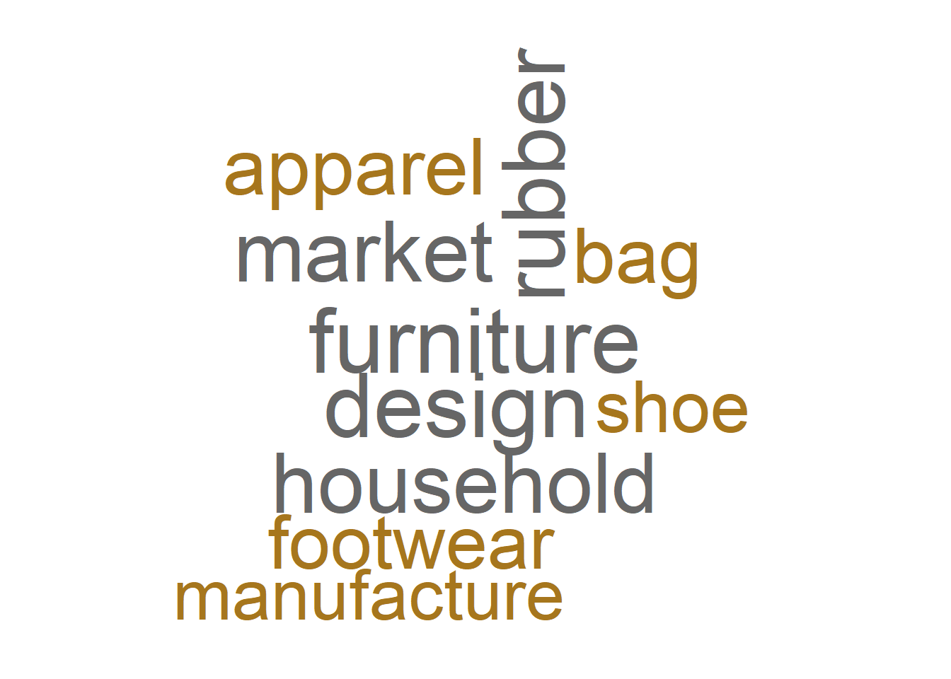
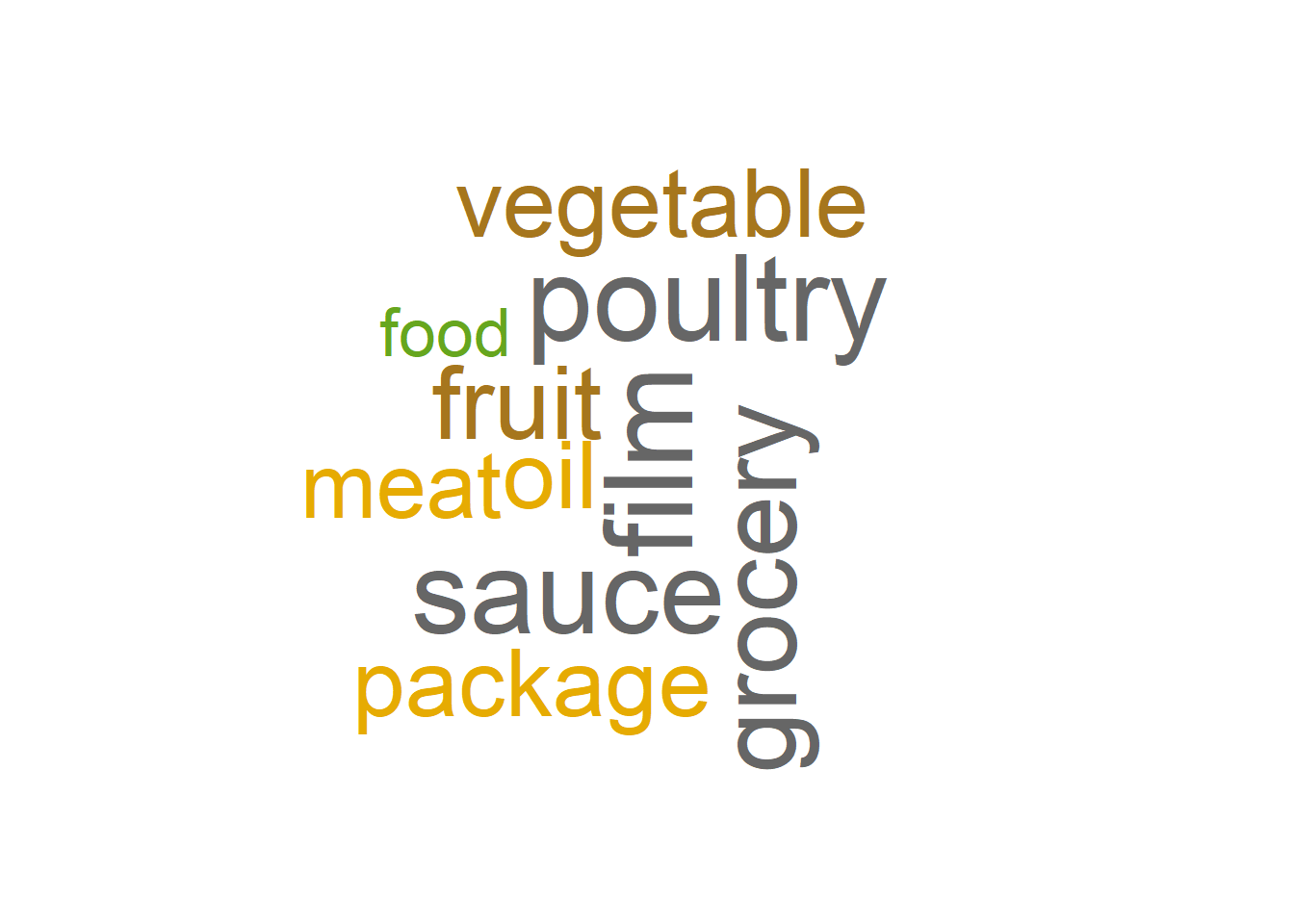
Below are the word clouds for each topic, representing the most frequent and significant words within each topic.
Topic 1 Keywords: machine, steel, cast, construction, power, metal, equipment Industry: Manufacturing of construction equipment, heavy machinery, metal fabrication Description: Companies may specialize in working with steel and casting, utilizing machinery and power for their operations.
Topic 2 Keywords: seafood, cod, tuna, fish, shellfish, marine, crab, fillet, salmon, shrimp Industry: Seafood processing and distribution, fishery, seafood restaurants Description: Company most likely involved in the seafood industry, specifically dealing with shrimp, salmon, fillet, shellfish, marine products, crab, cod, seafood, fish, and tuna. They may be engaged in activities such as fishing, processing, and selling various types of seafood products.
Topic 3 Keywords: freight, cargo, truck, storage, air, sea, transport, warehouse, container Industry: Freight transportation, logistics, warehousing, shipping Description: Companies may specializes in cargo handling and storage solutions, offering efficient air, sea, and truck transportation services. They provide reliable shipping and delivery options, including container logistics and warehouse management. Their expertise lies in facilitating the smooth movement of goods, ensuring timely and secure transportation throughout the supply chain.
Topic 4 Keywords: shoe, apparel, bag, design, rubber, furniture, market, household, footwear, manufacture Industry: Fashion and apparel manufacturing, shoe production, design, retail Description: Companies may operate in the retail or consumer goods industry. “rubber” could indicate that the company uses or specializes in rubber-based materials or products. It appears that the company’s business revolves around the production or sale of consumer goods, particularly in the fashion and home furnishing sectors.
Topic 5 Keywords: package, poultry, meat, grocery, film, fruit, food, sauce, vegetable Industry: Food packaging, poultry and meat processing, grocery retail Description: Companies involved in the production, packaging, and distribution of various food products.
Topic 6 Keywords: textile, paper, water, finish, paint, glue, fiber, light, base, fabric Industry: Textile manufacturing, paper production, adhesive and glue manufacturing

terms <- topicModel@terms
beta <- topicModel@beta

# Number of words to show for each topic
n_words <- 10

# Create a word cloud for each topic
for (k in 1:6) {
  prob <- beta[k, ]
  words <- terms[order(prob, decreasing = TRUE)][1:n_words]
  prob <- prob[order(prob, decreasing = TRUE)][1:n_words]
  prob <- prob / sum(prob)
  df <- data.frame(word = words, freq = prob)
  wc <- wordcloud(words = df$word, freq = df$freq, min.freq = 1,
            max.words = n_words, scale=c(4, 0.3), random.order = FALSE, rot.per = 0.35, colors = brewer.pal(8, "Dark2"), main = paste("Topic", k))
  plot_list[[k]] <- wc
}
grid_arrange <- grid.arrange(grobs = plot_list, nrow = 4, ncol = 3)
grid.draw(grid_arrange)
Assign topic to each company
Show code
topic_word_probs <- tidy(topicModel, matrix = "beta")
token_topic_words <- token_nodes_table %>%
  unnest_tokens(word,
                product_services)
company_topics <- left_join(token_topic_words, topic_word_probs, by = c("word" = "term"))
company_topics <- company_topics %>%
  group_by(id) %>%
  top_n(1, beta) %>%
  ungroup() %>%
  select(id, topic, beta)
company_topics <- unique(company_topics)
token_nodes_table$topic <- company_topics$topic
token_nodes_table$TopicLabel <- ifelse(token_nodes_table$topic == 1, "Manufacturing and Construction Equipment", ifelse(token_nodes_table$topic == 2, "Seafood processing and distribution, fishery, seafood restaurants", ifelse(token_nodes_table$topic == 3, "Freight transportation, logistics, warehousing, shipping", ifelse(token_nodes_table$topic == 4, "Fashion and Apparel Industry", ifelse(token_nodes_table$topic == 5, "Food packaging and Grocery Industry", "Textile and Paper Industry")))))

topic_map <- token_nodes_table %>%
  select(id, TopicLabel)
DT::datatable(topic_map)
Distribution of companies in each topic
topic_counts <- table(token_nodes_table$TopicLabel)
topic_counts_df <- data.frame(topic = names(topic_counts), count = as.numeric(topic_counts)) %>%
  mutate(topic = reorder(topic, count))
bar_plot <- ggplot(topic_counts_df, aes(x = topic, y = count)) +
  geom_bar(stat = "identity", fill = "steelblue") +
  labs(y = "Count", title = "Topic Distribution") +
  theme_minimal() +
  coord_flip() +
  xlab(NULL)
ggplotly(bar_plot)
Unveiling Industry Insights
Exploring Revenue Distribution Across Diverse Sectors
Observation:
In our analysis of different industries, we examined the median revenue for each industry. The manufacturing and construction equipment industry stood out with the highest median revenue, reaching approximately 34,000 omu. This industry’s strong performance can be attributed to its focus on producing machinery, steel casting, and utilizing power for construction purposes.
Following closely behind is the freight and logistics industry, which boasts a median revenue of 33,000 omu. This industry is involved in the transportation and storage of goods, both by air and sea. Its pivotal role in facilitating trade and commerce contributes to its solid revenue figures.
Not far behind is the food packaging and grocery industry, with a median revenue of 32,000 omu. This sector specializes in packaging food products, ensuring their quality and preservation. It also includes the grocery segment, offering a wide range of food items to consumers.
In the fourth position is the textile and paper industry, with a median revenue of 28.6 thousand omu. This industry is involved in the production of textiles, paper products, and related materials. It plays a vital role in the manufacturing and supply chain of various consumer goods.
On the other end of the spectrum, we find the seafood industry with a median revenue of 27,000 omu. This industry focuses on the harvesting, processing, and distribution of seafood products, meeting the demand for fresh and high-quality seafood.
Lastly, we have the fashion and apparel industry, which also showcases a median revenue of 27,000 omu. This sector encompasses the design, manufacturing, and retail of clothing and accessories, catering to fashion-conscious consumers.
These findings shed light on the revenue distribution across different industries. It’s clear that the manufacturing and construction equipment industry leads the way, followed closely by freight and logistics, and food packaging and grocery.
revenue_business_group <- inner_join(topic_map, mc3_nodes, by = "id")
revenue_business_group <- revenue_business_group %>%
  select(id, country, type, revenue_omu, TopicLabel) %>%
  na.omit()

##remove outliers for each topic label
fences <- revenue_business_group %>%
  group_by(TopicLabel) %>%
  summarise(lower_fence = quantile(revenue_omu, 0.25) - 1.5 * IQR(revenue_omu),
            upper_fence = quantile(revenue_omu, 0.75) + 1.5 * IQR(revenue_omu))

# Remove outliers for each TopicLabel
filtered_revenue_business_group <- revenue_business_group %>%
  left_join(fences, by = "TopicLabel") %>%
  filter(revenue_omu >= lower_fence, revenue_omu <= upper_fence) %>%
  select(id, country, type, revenue_omu, TopicLabel)

p <- ggplot(filtered_revenue_business_group, aes(x = reorder(TopicLabel, desc(revenue_omu)), y = revenue_omu, fill = TopicLabel)) +
  geom_boxplot() +
  labs(x = "Topic Label", y = "Revenue") +
  theme_minimal() +
  coord_cartesian(ylim = c(0, 300000))
p <- p + theme(axis.text.x = element_text(angle = 45, hjust = 0.5, vjust = 0.5))

ggplotly(p)
Unveiling Industry Titans
Exploring Dominant Players Across Countries
Observation:
In the fashion and apparel industry, Osterivaria emerges as a dominant force, contributing to 52.4% of the total revenue. This country’s fashion industry thrives, showcasing its strong market presence and capturing a significant share of the industry’s revenue.
Moving on to the food packaging and grocery industry, Utoporiana takes the lead, accounting for a substantial 66% of the revenue. This country’s efficient packaging and grocery sector plays a pivotal role in meeting consumer demands and driving revenue growth.
When it comes to the freight and logistics industry, Isliandor emerges as a major player, contributing to 43.2% of the total revenue. The country’s well-established logistics infrastructure and strategic location position it as a hub for transportation and storage, attracting significant business activity.
In the manufacturing and construction equipment industry, Alverovia stands out with a significant market share, accounting for 29.8% of the revenue. The country’s expertise in manufacturing and construction-related machinery and equipment contributes to its strong performance in this industry.
The seafood industry showcases a clear leader, with ZH dominating the market and accounting for a remarkable 72.25% of the revenue. This country’s abundant marine resources and expertise in seafood processing and distribution solidify its position as a key player in the global seafood market.
Finally, in the textile and paper industry, ZH once again takes the spotlight, accounting for 35.9% of the total revenue. The country’s advanced textile manufacturing capabilities and robust paper production sector contribute to its significant revenue share.
These findings highlight the prominent role played by specific countries in each industry, showcasing their expertise, market dominance, and revenue contribution. Understanding the big players in various industries provides valuable insights into global market dynamics and helps identify potential areas for collaboration and investment.
cluster_avg_revenue <- revenue_business_group %>%
  group_by(TopicLabel,country) %>%
  summarise(avg_revenue = mean(revenue_omu))
# Plot the stacked bar plot
p <- ggplot(cluster_avg_revenue, aes(x = TopicLabel, y = avg_revenue, fill = country)) +
  geom_bar(stat = "identity") +
  labs(x = "Cluster", y = "Average Revenue") +
  scale_fill_discrete(name = "Country") +
  theme_minimal()+
  theme(legend.position = "bottom", axis.text.x = element_text(angle = 45, hjust = 0.5, vjust = 0.5))

 p <- p + scale_y_continuous(labels = comma)


ggplotly(p)
References
LADAL. (n.d.). Topic Modeling. Language and Document Analysis Lab. Retrieved from https://ladal.edu.au/topicmodels.html